Semi-Intrusive von Karman Shell
Contents
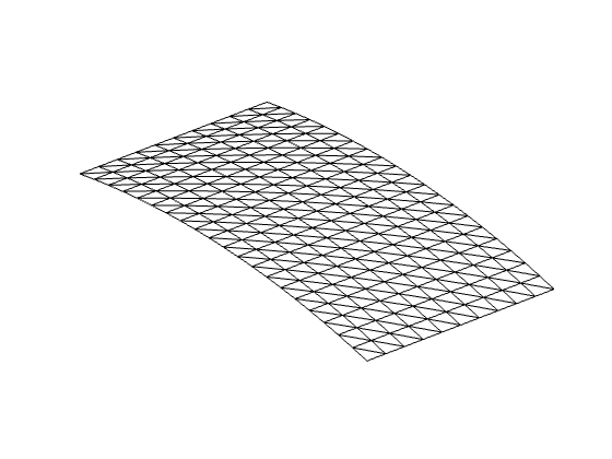
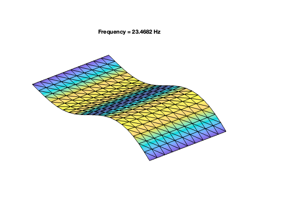
Shallow-curved shell structure with geometric nonlinearities
Finite element model used in the following reference:
Jain, S., & Tiso, P. (2018). Simulation-free hyper-reduction for geometrically nonlinear structural dynamics: a quadratic manifold lifting approach. Journal of Computational and Nonlinear Dynamics, 13(7), 071003. <https://doi.org/10.1115/1.4040021>
Finite element code taken from the following package:
Jain, S., Marconi, J., Tiso P. (2020). YetAnotherFEcode (Version v1.1). Zenodo. <http://doi.org/10.5281/zenodo.4011282>
clear all; close all; clc
run ../../install.m
% change to example directory
exampleDir = fileparts(mfilename('fullpath'));
cd(exampleDir)
system parameters
nDiscretization = 10; % Discretization parameter (#DOFs is proportional to the square of this number)
epsilon = 0.1;
generate model
[M,C,K,fnl,dfnl,f_0,outdof] = build_model_semiIntrusive(nDiscretization);
n = length(M); % number of degrees of freedom
disp(['Number of degrees of freedom = ' num2str(n)])
disp(['Phase space dimensionality = ' num2str(2*n)])
Building FE model
Assembling M,C,K matrices
Applying boundary conditions
Solving undamped eigenvalue problem
Using Rayleigh damping
Assembling external force vector
Total time spent on model assembly = 00:00:01
Number of degrees of freedom = 1320
Phase space dimensionality = 2640


Dynamical system setup
We consider the forced system
which can be written in the first-order form as
where
.
DSorder = 2;
DS = DynamicalSystem(DSorder);
set(DS,'M',M,'C',C,'K',K,'fnl_semi',fnl,'dfnl_semi',dfnl);
set(DS.Options,'Emax',5,'Nmax',10,'notation','multiindex')
set(DS.Options,'Intrusion','semi')
% set(DS.Options,'Emax',5,'Nmax',10,'notation','tensor')
We assume periodic forcing of the form
Fourier coefficients of Forcing
kappas = [-1; 1];
coeffs = [f_0 f_0]/2;
DS.add_forcing(coeffs, kappas,epsilon);
Linear Modal analysis and SSM setup
[V,D,W] = DS.linear_spectral_analysis();
Due to high-dimensionality, we compute only the first 5 eigenvalues with the smallest magnitude. These would also be used to compute the spectral quotients
Assuming a proportional damping hypthesis with symmetric matrices
modal damping ratio for 1 mode is 2.000000e-03
modal damping ratio for 2 mode is 2.000000e-03
modal damping ratio for 3 mode is 2.269789e-03
modal damping ratio for 4 mode is 2.721500e-03
modal damping ratio for 5 mode is 2.909530e-03
the left eigenvectors may be incorrect in case of asymmetry of matrices

 The first 10 nonzero eigenvalues are given as
   1.0e+02 *

  -0.0029 + 1.4745i
  -0.0029 - 1.4745i
  -0.0063 + 3.1598i
  -0.0063 - 3.1598i
  -0.0094 + 4.1319i
  -0.0094 - 4.1319i
  -0.0148 + 5.4515i
  -0.0148 - 5.4515i
  -0.0173 + 5.9601i
  -0.0173 - 5.9601i
Choose Master subspace (perform resonance analysis)
S = SSM(DS);
set(S.Options, 'reltol', 0.1,'notation','multiindex')
% set(S.Options, 'reltol', 0.1,'notation','tensor')
masterModes = [1,2];
S.choose_E(masterModes);
(near) outer resonance detected for the following combination of master eigenvalues
     4     0
     0     4

These are in resonance with the follwing eigenvalues of the slave subspace
   1.0e+02 *

  -0.0173 + 5.9601i
  -0.0173 - 5.9601i

sigma_out = 5
(near) inner resonance detected for the following combination of master eigenvalues
     2     1
     3     2
     1     2
     2     3

These are in resonance with the follwing eigenvalues of the master subspace
   1.0e+02 *

  -0.0029 + 1.4745i
  -0.0029 + 1.4745i
  -0.0029 - 1.4745i
  -0.0029 - 1.4745i

sigma_in = 5
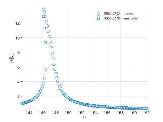
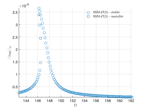
Forced response curves using SSMs
Obtaining forced response curve in reduced-polar coordinate
order = 3; % Approximation order
setup options
set(S.Options, 'reltol', 1,'IRtol',0.02,'notation', 'multiindex','contribNonAuto',false,'COMPtype','first')
set(S.FRCOptions, 'nt', 2^7, 'nRho', 200, 'nPar', 200, 'nPsi', 100, 'rhoScale', 2 )
set(S.FRCOptions, 'method','level set')
%set(S.FRCOptions, 'method','continuation ep', 'z0', 1e-4*[1; 1]) % 'level set'
set(S.FRCOptions, 'outdof',outdof)
choose frequency range around the first natural frequency
omega0 = imag(S.E.spectrum(1));
omegaRange = omega0*[0.9 1.1];
extract forced response curve
FRC = S.extract_FRC('freq',omegaRange,order);
figFRC = gcf;
*****************************************
Calculating FRC using SSM with master subspace: [1  2]
(near) outer resonance detected for the following combination of master eigenvalues
     2     0
     3     0
     3     1
     4     1
     0     2
     0     3
     1     3
     1     4
     2     0
     3     0
     3     1
     4     1
     0     2
     0     3
     1     3
     1     4
     3     0
     4     0
     4     1
     0     3
     0     4
     1     4
     4     0
     5     0
     0     4
     0     5

These are in resonance with the follwing eigenvalues of the slave subspace
   1.0e+02 *

  -0.0063 + 3.1598i
  -0.0063 + 3.1598i
  -0.0063 + 3.1598i
  -0.0063 + 3.1598i
  -0.0063 - 3.1598i
  -0.0063 - 3.1598i
  -0.0063 - 3.1598i
  -0.0063 - 3.1598i
  -0.0094 + 4.1319i
  -0.0094 + 4.1319i
  -0.0094 + 4.1319i
  -0.0094 + 4.1319i
  -0.0094 - 4.1319i
  -0.0094 - 4.1319i
  -0.0094 - 4.1319i
  -0.0094 - 4.1319i
  -0.0148 + 5.4515i
  -0.0148 + 5.4515i
  -0.0148 + 5.4515i
  -0.0148 - 5.4515i
  -0.0148 - 5.4515i
  -0.0148 - 5.4515i
  -0.0173 + 5.9601i
  -0.0173 + 5.9601i
  -0.0173 - 5.9601i
  -0.0173 - 5.9601i

sigma_out = 5
(near) inner resonance detected for the following combination of master eigenvalues
     2     1
     3     2
     1     2
     2     3

These are in resonance with the follwing eigenvalues of the master subspace
   1.0e+02 *

  -0.0029 + 1.4745i
  -0.0029 + 1.4745i
  -0.0029 - 1.4745i
  -0.0029 - 1.4745i

sigma_in = 5
Due to (near) outer resonance, the exisitence of the manifold is questionable and the underlying computation may suffer.
Attempting manifold computation
Manifold computation time at order 2 = 00:00:00
Estimated memory usage at order  2 = 2.23E+00 MB
Manifold computation time at order 3 = 00:00:00
Estimated memory usage at order  3 = 2.39E+00 MB
gamma =
  -7.2120e+00 - 2.9595e+02i

Total time spent on FRC computation upto O(3) = 00:00:02


